Literature Overview

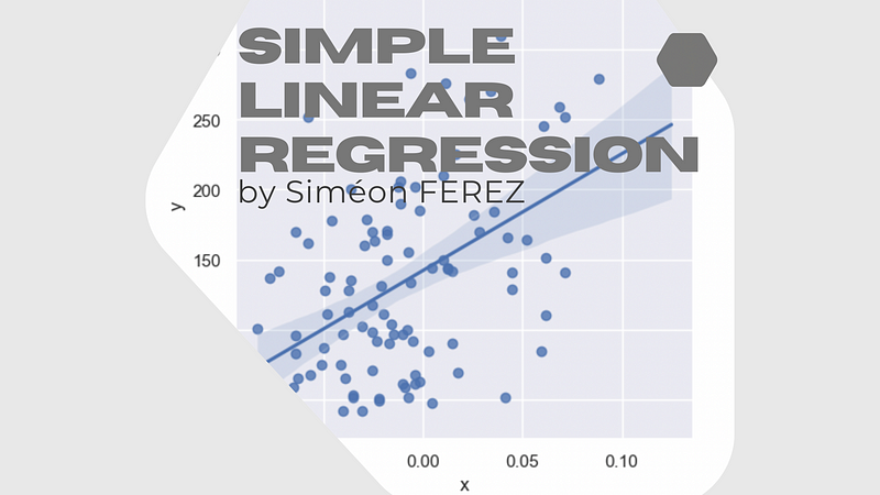
In this exploration, we will concentrate solely on simple linear regression as opposed to multiple linear regression, which will be explored in subsequent projects. Simple linear regression is aimed at predicting a single output value based on the relationship between input data points. The core principle involves fitting a line to the data, expressed through an equation such as:

In this equation:

• ?: represents the slope of the line
• ?: denotes the intercept

Recognizing that our input data may not be flawless and could include noise—due to sensor inaccuracies or data conversion issues—we depict the error for each point as shown below:

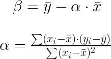
The linear regression process aims to identify the best-fitting line while minimizing the squared error across all points. This involves solving the least-squares problem to determine the parameters ? and ? that reduce this error.

Methodological Approach

For computation, we employ Python's linear regression capabilities, utilizing libraries such as pandas, NumPy, Matplotlib, Seaborn, and Scikit-learn. The code is structured into various sub-functions, each responsible for specific tasks—such as reading the CSV file, calculating coefficients, and plotting results—while a main function orchestrates these sub-functions.

Our initial step involves exploring the input dataset:

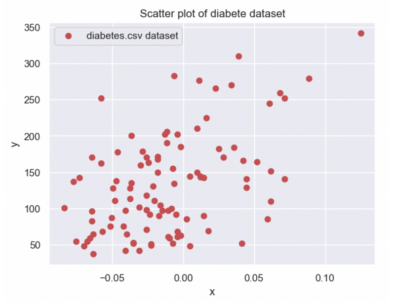
This scatter plot provides an initial assessment, indicating that our slope coefficient ? is likely between 500 and 1000, with the intercept ? around 150. This preliminary data helps in validating our coefficient calculations.

Results of Calculation

After performing manual calculations, I determined ? = 831.767374 and ? = 142.327327, values that align with our earlier visual analysis. Additionally, I represented the equation of the line y = ?x + ? using the input dataset.

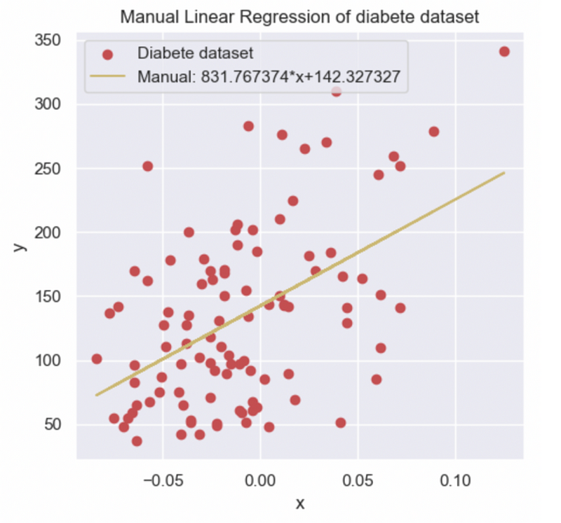
To further validate my findings, I utilized the Scikit-learn library's LinearRegression() function, plotting the results against my manual calculations for comparison.

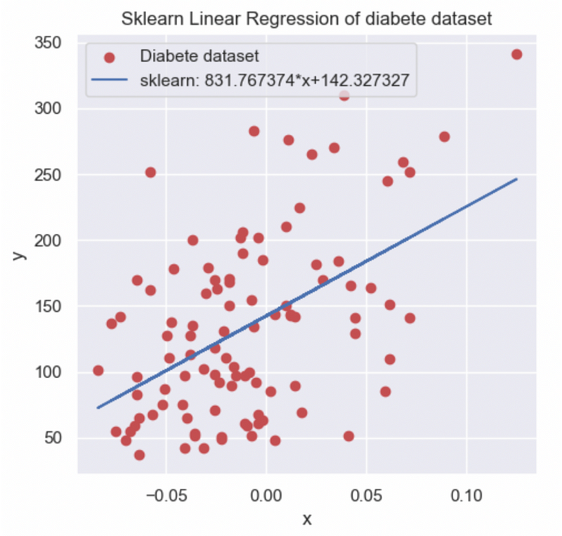
Ultimately, both methods yielded identical coefficients. To enhance validation and evaluation of my linear regression model, I computed various metrics to analyze its accuracy and performance.

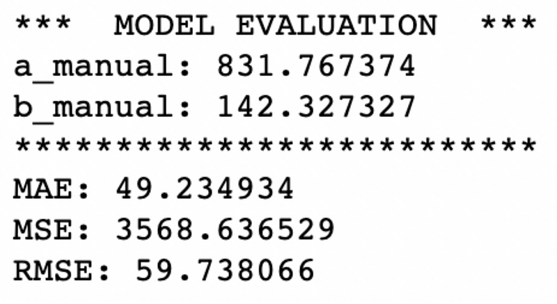
The Mean Absolute Error (MAE) represents the average deviation of our model's predictions from the actual values, compared to the average value of y(x), which is 133.56. This indicates that our model still exhibits significant error. The Mean Squared Error (MSE) penalizes larger discrepancies more heavily, thus producing a higher value than MAE due to the presence of noise and outliers in the dataset.

Sample Code for Coefficient Calculation

def compute_sklearn(df):

# Function to calculate coefficients a & b using the sklearn library

# Parameters:

# - df: Pandas DataFrame created from the diabetes.csv dataset

# The DataFrame contains columns "x" and "y"

# Returns the coefficients a & b

sk_x = df["x"].values.reshape(-1, 1)

sk_y = df["y"].values.reshape(-1, 1)

linear_regression = LinearRegression()

linear_regression.fit(sk_x, sk_y)

return linear_regression.coef_[0][0], linear_regression.intercept_[0] # Returns parameters a & b

def compute_coeffs(df):

# Function to calculate coefficients a & b through manual computation

# Parameters:

# - df: Pandas DataFrame created from the diabetes.csv dataset

# The DataFrame contains columns "x" and "y"

# Returns coefficients a & b

sum1, sum2 = 0, 0

xmean = np.mean(df['x'])

ymean = np.mean(df['y'])

for index, row in df.iterrows():

sum1 += (row['x'] - xmean) * (row['y'] - ymean)

sum2 += (row['x'] - xmean) ** 2

return sum1 / sum2, ymean - (sum1 / sum2) * xmean